Gaussian Mixture Models and Cluster Membership
Applying Gaussian Mixture Models to Gaia Data
In my research, I look for planets around stars in a certain type of star cluster known as a globular cluster. Globular clusters are the oldest known star clusters and are nearly as old as the universe. Although the locations of many of these clusters are well known and documented, interloping stars that happen to be in the same area of the sky as these clusters are always present in telescope images. This makes it difficult to know which stars in an image actually belong to the cluster. We have to figure out after the fact which stars belong to the cluster and which do not, often by using additional data.
There are several methods, all data-driven, that can be used to determine cluster membership. None of these methods work for all clusters, so the ideal membership classification method has to be determined cluster by cluster. Fortunately for the cluster I am working on right now, there is one method that performs very well—the proper motion method—and there is a public data set that was recently released that has all the data necessary to use this method.
The Proper Motion Method
First, let me define “proper motion.” Stars appear fixed relative to each other in the sky, but this is only an illusion. All stars are in motion relative to Earth, but they are all so far away that, except for a few stars, this motion is imperceptible to naked-eye observations over millenium-long timescales. However, with precise instruments and enough time, the motion of stars across the sky can be detected and measured. The motion of a star on the plane of the sky is called its “proper motion.” (A second type of stellar motion, “radial velocity”, is the motion of the star towards or away from Earth, perpendicular to the plane of the sky, but the technique to measure this motion is quite different than that used to measure proper motion.) The magnitude of measured proper motions is usually on the order of 1–10 milliarcseconds per year. A milliarcsecond is 1 / 3,600,000 of a degree, just to get an idea of how incredibly small these motions on the sky are.
Most stars move randomly relative to each other, and thus proper motions are (very nearly) random. However, stars in a star cluster move together (otherwise they wouldn’t be clustered!) and so their proper motions are not random relative to each other. Additionally, some star clusters (including the one I am most interested in in my research) have higher than normal proper motions. It is these characteristics—similar proper motions for cluster stars that are distinct from non-cluster stars—that make proper motion data useful to distinguish which stars belong to my cluster and which just happen to be in the same area of the sky.
The Data Set
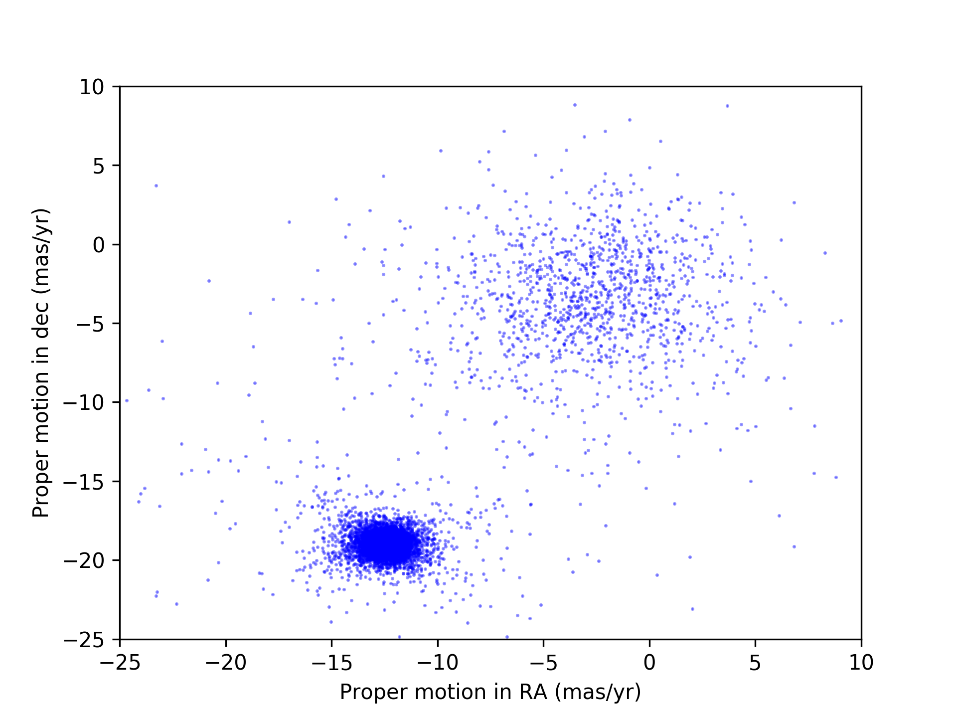
The proper motion data I used for this analysis were obtained with the Gaia satellite, an incredible spacecraft with an ambitious mission to obtain proper motions for over a billion stars, by far the largest such dataset ever assembled. The first data release from this mission, in 2016, was only a partial data release and didn’t have proper motions for most of the stars I am analyzing. Thus, I had to wait for the second data release in April 2018, which contains a much more complete set of proper motions and includes the stars I need. The figure below shows the proper motions measured for stars in a section of sky in the direction of the cluster I’m studying.

Globular Cluster Proper Motion
Proper motions for stars in the direction of the globular cluster M4. RA stands for right ascension and dec stands for declination, which are two axes that, respectively, run east–west and north–south on the sky; mas stands for milliarcsecond.
As we can see, there are two clumps of points: one centered roughly on (-2, -5), and a second, more concentrated clump centered roughly on (-13, -20). It is this second, more concentrated clump that is the stars that belong to the star cluster and is consistent with previously measured values for the cluster. So, yay! We have a robust data set with very distinct clustering that allows for accurate classification. What next though? How do we use the data to calculate a cluster membership probability, preferably in an automated way? There’s more than one way to skin this cat, and the way I chose is to use a Gaussian mixture model.
Gaussian Mixture Models
Mixture models work with “mixed” datasets, which are datasets that can be described as mixtures of two or more distinct subsets of the data. The population of passengers at a train station is an example of such a dataset. It consists of three subpopulations: those who came from outside the station to get on a train, those leaving the station after getting off a train, and those who are making a train after getting off another train. (This ignores, e.g., people waiting to meet people coming off a train, but I’m ignoring these for simplicity.) These three subpopulations are mixed together, but with the right data could be separated out despite the mixture.
Mixture models assume that there is an underlying latent substructure to the dataset and then uses the data itself to discover this substructure. This discovered substructure can then be used to determine the membership of a data point in a given subpopulation. Such membership determinations are not deterministic though, which is one of the advantages of mixture models. Instead, membership probabilities for all the subpopulations are determined. In the train station example above, if we were able to interview everybody in the train station and they were all honest, then we would have sufficient data to determine exactly to which of the three subpopulations everybody belonged. If, though, we weren’t able to obtain such high-quality data and only had, say, a knowledge of their current location in the train station, then at best we could only determine the probability a person had of belonging to each of the subpopulations.
The particular flavor of mixture model I chose to use was the Gaussian mixture model (GMM). This model assumes that the data arise from a mixture of Gaussian-distributed subpopulations. A specified number of Gaussian distributions are then fit to the data, with their means and variances being the parameters that are fit (typically using the expectation-maximization algorithm to maximize the likelihood).
Why did I choose a GMM instead of another type of mixture model? First, eyeballing the data in Figure 1, the clustering of the data looks at least Gaussian-ish: two dense, central cores with point density tapering off from the cores with roughly elliptical contour lines. Second, the proper motions of the objects belonging to the star cluster are randomly distributed relative to the bulk motion of the cluster. I didn’t check formally whether one would expect this random distribution to be Gaussian, but my intuition of the dynamics of globular clusters suggests that a Gaussian is at least a good approximation if not the exact answer. Third, the measurement errors (which are about 20% the size of the stars’ proper motions relative to the cluster’s bulk proper motion, so significant) should be Gaussian if there are no systematic errors, which also makes the point distribution tend towards a Gaussian shape. Thus a Gaussian seems a very reasonable guess to make. One can also check this guess by plotting up histograms of the proper motions in both directions, which I did and verified that they are quite Gaussian (though the non-cluster clump of points is asymmetric in declination; more on this later).
The Results
Let’s see how well the GMM works. I used the scikit-learn package’s mixture.GaussianMixture for this.

Cluster Membership Probabilities Using A GMM
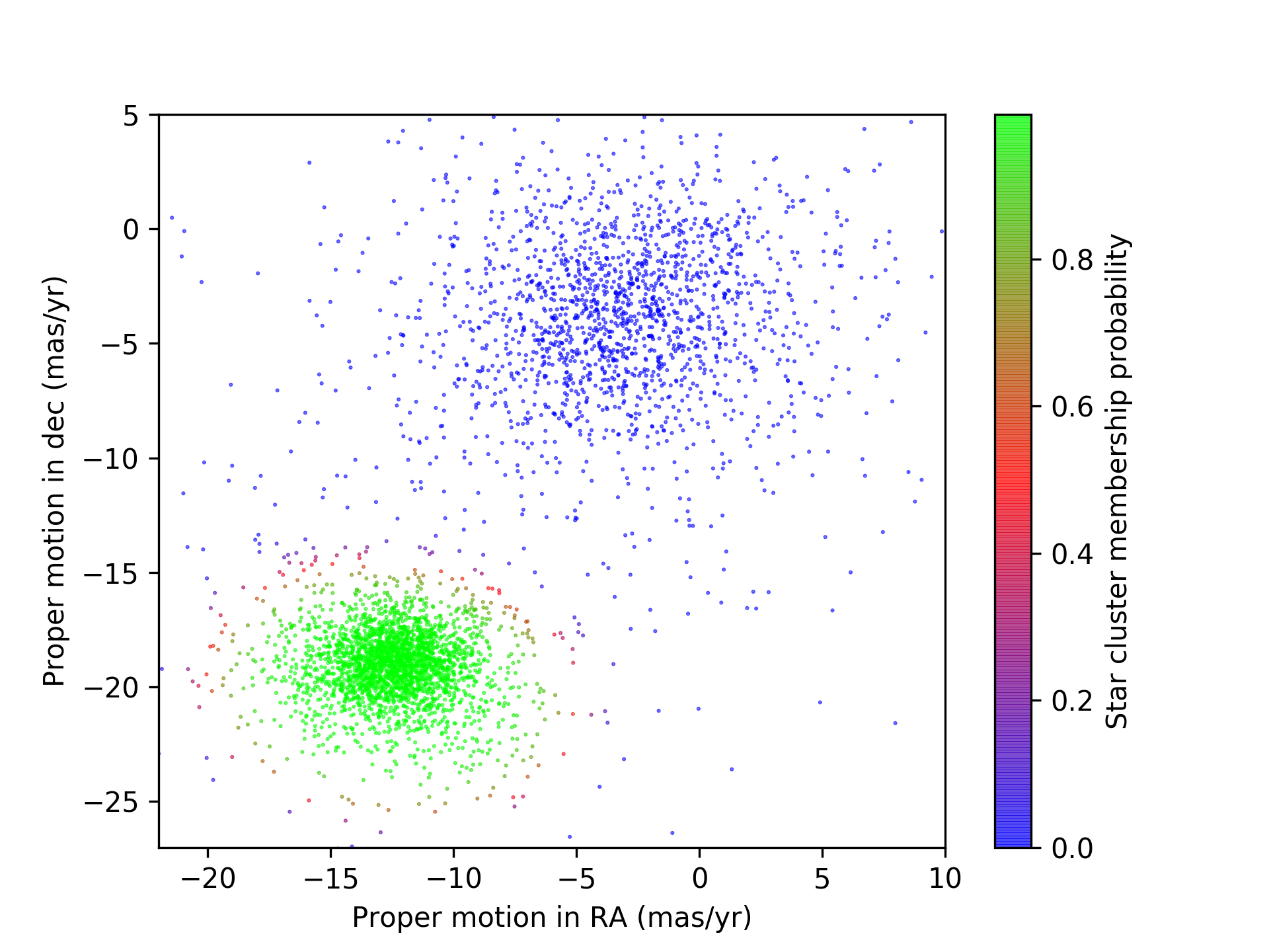
Proper motions for stars in the direction of the globular cluster M4, with cluster membership probabilities calculated by fitting a GMM. Green denotes high probability of cluster membership while blue denotes low probability of membership and red denotes ambiguous membership. Note that this is zoomed in relative to the previous figure.
I think the GMM did very well, especially considering how fast it was to implement and that there was no need to optimize hyperparameters. The model has discovered and separated the two clusters. One important note is that mixture models identify clusters in the data but do not attach any sort of “labels” to the cluster; labels have to be assigned after the fact. Relatedly, different initializations for the the model fitting can lead to correct but inverted cluster identification. In the present case, what is stored in the output as “the second of the two clusters” that the model discovered is the correct cluster, but with a different initialization the correct cluster may end up as “the first of the two clusters” in the output. This must be minded if you care about labelling your clusters and end up rerunning the code with a different initialization.
One thing I notice is that the red points, with equal probability of belonging to either cluster, seem more likely to belong to the green point cluster based on the density of points in the vicinity. A possible cause of this is the (small) asymmetry I found in the distribution of the proper motions in declination for the non-cluster members stars.
Conclusion
Using a GMM for cluster membership determination has been extremely useful in my research. The power of this incredible dataset from the Gaia mission, coupled with a simple yet robust clustering algorithm, has allowed a relatively small amount of effort to produce a cluster membership catalog that is better than anything previously published. That just goes to show that with a large enough dataset of good quality, previously elusive answers can be easily discovered.

Share this post
Twitter
Facebook
LinkedIn
Email